知识清单

• 二项分布

  • 性质
  • 应用

• Poison分布

  • 性质
  • 应用

• 负二项分布

  • 性质
  • 应用

1. 二项分布

二项分布（binomial distribution），是指只有两种可能结果的n此独立重复实验中，出现阳性次数X的一种概论分布

1.1 适用条件

• 每次试验只会发生两种对立的可能结果之一，即分别发生两种结果的概率之和恒为1

• 每次试验产生某种结果（如“阳性”）的概率固定不变

• 重复试验是独立的

1.2 性质

• X的均数与方差

 
​x
\mu = n\pi  
​
\sigma^2 = n\pi(1-\pi)

• 率p的均值和方差

 
xxxxxxxxxx
\mu_{p} = \pi
​
\sigma_{p}^2 = \frac{\pi(1-\pi)}{n}

• n -> 无穷大，而pi不太靠近0或1时，二项分布近似正态分布；n -> 无穷大，而pi靠近0时，二项分布近似Poision分布

1.3 应用

1.3.1 总体率的区间估计与假设检验（精确检验）

n<=50的小样本只能直接查表（如13名手术患者进行治疗，6人痊愈，估计其痊愈率的95%可信区间，并与一疗效为50%的治疗方案有无差异？）

 
xxxxxxxxxx
# 数据
> ratio <- 6/13
> x <- 6
> n <- 13
# 检验
> library(Hmisc)
> binconf(x, n, alpha=0.05, method="exact")
  PointEst     Lower     Upper
 0.4615385 0.1922324 0.7486545
> binconf(x, n, alpha=0.05, method="wilson")
  PointEst     Lower    Upper
 0.4615385 0.2320607 0.708562
> binconf(x, n, alpha=0.05, method="all")
            PointEst     Lower     Upper
Exact      0.4615385 0.1922324 0.7486545
Wilson     0.4615385 0.2320607 0.7085620
Asymptotic 0.4615385 0.1905457 0.7325312
> 
> binom.test(x, n, p = 0.5,
+            alternative = "two.sided",
+            conf.level = 0.95)
​
    Exact binomial test
​
data:  x and n
number of successes = 6, number of trials = 13, p-value = 1
alternative hypothesis: true probability of success is not equal to 0.5
95 percent confidence interval:
 0.1922324 0.7486545
sample estimates:
probability of success 
             0.4615385 

参考：
https://stat.ethz.ch/R-manual/R-devel/library/stats/html/binom.test.html
https://stackoverflow.com/questions/21719578/confidence-interval-for-binomial-data-in-r
n较大、p和1-p均不太小，np和n(1-p)均大于5时，可近似正态分布

 
xxxxxxxxxx
N(\pi, \sigma_{p}^2)

计算1-alpha的可信区间可以近似为：

 
xxxxxxxxxx
(p - u_{\alpha/2}S_{p}, p + u_{\alpha/2}S_{p})

如100人接受药物治疗后55人有效，估计有效率95%可信区间

 
xxxxxxxxxx
> x <- 55
> n <- 100
> Sp <- sqrt(x/n*(1-x/n)/n)
> x/n + c(-1, 1)*qnorm(p=0.975)*Sp
[1] 0.452493 0.647507
> library(Hmisc)
> binconf(x, n, alpha=0.05, method="all")
           PointEst     Lower     Upper
Exact          0.55 0.4472802 0.6496798
Wilson         0.55 0.4524460 0.6438546
Asymptotic     0.55 0.4524930 0.6475070
> binom.test(x, n, 0.5,
+            alternative="two.sided",
+            conf.level=0.95)
​
    Exact binomial test
​
data:  x and n
number of successes = 55, number of trials = 100, p-value = 0.3682
alternative hypothesis: true probability of success is not equal to 0.5
95 percent confidence interval:
 0.4472802 0.6496798
sample estimates:
probability of success 
                  0.55 

1.3.2 样本率与总体率的比较

直接法

分单侧（优或劣问题）和双侧（是否相同问题），这两种情况的算法截然不同【但是单侧和双侧的基本思想与t检验这些都相同的， 即双侧检验计算小于当前事件概率的所有小概率事件之和得出p值，单侧检验计算小于当前事件并且值大于或者小于当前X值的事件概率之和得出p值】，下面以例题代码演示

• 单侧检验

 
xxxxxxxxxx
# 单侧检验
# 例：手术方式1的成功率为0.55
#     手术方式2进行试验，10例成功9例
# 问：手术方式2是否优于手术方式1？
# H0为手术方式2的成功率=0.55
# H1为手术方式2的成功率高于0.55
​
# 绘图代码
size = 10  # 独立重复试验次数
prob = 0.55  # 每次成功的概率
test_x = 9  # 实际成功次数
x_range <- seq(0, size, by=1)
p_range <- dbinom(prob=prob, size=size, x=x_range)
data <- data.frame(x_range=x_range,
  p_range=p_range, 
  test_type =factor(
    as.numeric(p_range<=(p_range[x_range==test_x]))+as.numeric(x_range>=test_x),
    levels=c(0, 1, 2), labels=c("not test", "left tail", "right tail")))
library(ggplot2)
p <- ggplot(data, aes(x_range, p_range, color=test_type))+geom_line(aes(x_range, p_range), color="gray55") + 
  geom_point(size=3) + geom_vline(aes(xintercept=test_x), color="blue", lwd=1, alpha=0.4) + 
  geom_hline(aes(yintercept=p_range[x_range==test_x]), color="green", lwd=1, alpha=0.4) +
  scale_x_continuous(breaks=x_range)+xlab("X")+ylab("Probability")+ggtitle(label=paste("X~B(", size, " ,", prob, ")", sep=""))+
  theme_classic()
p

 
xxxxxxxxxx
> # 单侧检验（优于0.55）p值计算
> # 即仅计算上图中右尾部分，为sum(P(X>=9))
> size = 10  # 独立重复试验次数
> prob = 0.55  # 每次成功的概率
> test_x = 9  # 实际成功次数
> x_range <- seq(0, size, by=1)
> p_range <- dbinom(prob=prob, size=size, x=x_range)
> p_value <- sum(p_range[x_range>=size])
> p_value
[1] 0.002532952

• 双侧侧检验
  把上题中的问题改为两种手术方法有无差异，则使用双侧检验，p值为sum(P(X=i)) where P(X=i) <= P(X=9)，而不是t检验中简单的单侧检验乘2，因为二项分布可能是不对称的

 
xxxxxxxxxx
> # 双侧p值计算
> # 计算上图中左尾和右尾概率之和，sum(P(X=i)) where P(X=i) <= P(X=9))
> size = 10  # 独立重复试验次数
> prob = 0.55  # 每次成功的概率
> test_x = 9  # 实际成功次数
> x_range <- seq(0, size, by=1)
> p_range <- dbinom(prob=prob, size=size, x=x_range)
> p_value <- sum(p_range[p_range<=p_range[x_range==test_x]])
> p_value
[1] 0.02775935

正态近似法

条件：n较大，p和1-p均不太小，np和n(1-p)均大于5，二项分布可近似正态分布，其u值计算公式为

 
xxxxxxxxxx
u=\frac{p-\pi_{0}}{\sqrt{\pi_{0}(1-\pi_{0})/n}}

1.3.3 两样本率的比较

条件：n1与n2均较大，p1、p2、1-p1和1-p2均不太小（n1p1、n1(1-p1)、n2p2、n2(1-p2)均大于5），可利用样本率的分布近似正态分布且独立两正态变量之差也服从正态分布的性质，采用近似正态法对两总体率进行统计检验，u的计算公式为：

 
xxxxxxxxxx
u=\frac{p_{1}-p_{2}}{S_{p_{1}-p_{2}}}
​
S_{p_{1}-p_{2}}=\sqrt{\frac{X_{1}+X_{2}}{n_{1}+n_{2}}(1-\frac{X_{1}+X_{2}}{n_{1}+n_{2}}(\frac{1}{n_{1}}+\frac{1}{n_{2}})}

1.3.4 非遗传疾病的家族聚集性

• clustering in families系指改疾病发生在家族成员间是否有传染性，如果没有传染性，则家族成员是否患病独立，否则存在家族聚集性
• 以相同成员数目n的家庭为样本，对每个家庭出现X个患者的概率分布是否服从二项分布进行检验，从而分析其聚集性
• 实际资料与二项分布进行拟和优度的卡方检验得出p值

1.3.5 做群检验

• 群检验目的：为了解决检验大批标本的阳性率问题
• 具体做法：把N个标本分为n个群，每个群m个标本，即N=n*m。检验每个群是否为阳性群（一旦检测到阳性就停止检测当前群），只有阴性群才需要检测所有标本，可以大大减少检测数目
• 通过阳性群率计算阳性率：假设受检的n个群中，X个群为阳性群，则X/n可作为阳性群率的估计，记每个标本阳性率为pi，则

 
xxxxxxxxxx
1-(1-\pi)^{m}=\frac{X}{n}

2. Poisson分布

Poisson分布是二项分布的一种极端情况，已发展为描述小概率事件发生规律的一种重要分布，如分析发病率低的非传染性疾病发病或人数分布等、单位时间或面积、空间某罕见事物的分布，对应概率为

 
xxxxxxxxxx
P(x)=\frac{e^{-\lambda}\lambda^{X}}{X!}

\lambda为总体均数，e=2.71828为一常数

2.1 适用条件

假定在某观测单位内，某事件（如“阳性”）平均发生次数为lambda，且规定改观测单位可等分为充分多的n粉，其样本计数为X(X=0, 1, 2,···)，则在满足该条件时，有X~P(lambda):

1. 普通性
   在充分小的观测单位上X的取值最多为1
2. 独立增量性
   每个观测单位上X的取值与前面各观测单位无关
3. 平稳性
   X的取值只与观测单位的大小有关，而与观测单位的位置无关，即每一次使用阳性发生的概率都应相同，为pi=lambda/x，这样阳性数X的取值只与重复试验的次数相关，为合计的阳性总数，可看作是大量独立试验的总结果

2.2 性质和图形

1. 总体均数与总体方差相等
2. n很大pi很小，且npi=lambda时，二项分布近似Poisson分布
3. lambda增大时，Poisson分布渐近正态分布，lambda>=20时可作为正态分布
4. Possion分布具有可加性（和正态分布类似），但不具有可乘性（可由X取值和均数，方差看出）
5. Poisson分布的图形，若lambda时整数，则在X=lambda和X=lambda-1处有最大概率

 
xxxxxxxxxx
lambda <- 1:6
x <- 1:(2*max(lambda+1))
data <- data.frame(x=rep(x, times=length(lambda)), 
                   lambda=factor(rep(lambda, each=length(x))), 
                   prob=dpois(x, rep(lambda, each=length(x))))
library(ggplot2)
ggplot(data, aes(x=x, y=prob, color=lambda, group=lambda))+
  geom_point(size=2)+geom_line(lwd=1)+
  scale_x_continuous(breaks=floor(seq(min(x), max(x), by=((max(x)-min(x))/20))))

2.3 Poisson分布的应用

2.3.1 总体均数的区间估计

查表法(X<=50)

例：1立升空气测得粉尘粒子数为21，估计改车间平均每立升空气粉尘颗粒的95%和99%可信区间

 
xxxxxxxxxx
> exactci::poisson.exact(21, plot=T, conf.level=0.95)
​
    Exact two-sided Poisson test (central method)
​
data:  21 time base: 1
number of events = 21, time base = 1, p-value < 2.2e-16
alternative hypothesis: true event rate is not equal to 1
95 percent confidence interval:
 12.99933 32.10073
sample estimates:
event rate 
        21 
​
> exactci::poisson.exact(21, plot=T, conf.level=0.99)
​
    Exact two-sided Poisson test (central method)
​
data:  21 time base: 1
number of events = 21, time base = 1, p-value < 2.2e-16
alternative hypothesis: true event rate is not equal to 1
99 percent confidence interval:
 11.06923 35.94628
sample estimates:
event rate 
        21 
​
> poisson.test(20, alternative="two.sided", conf.level=0.95)
​
    Exact Poisson test
​
data:  20 time base: 1
number of events = 20, time base = 1, p-value < 2.2e-16
alternative hypothesis: true event rate is not equal to 1
95 percent confidence interval:
 12.21652 30.88838
sample estimates:
event rate 
        20 
​
> poisson.test(20, alternative="two.sided", conf.level=0.99)
​
    Exact Poisson test
​
data:  20 time base: 1
number of events = 20, time base = 1, p-value < 2.2e-16
alternative hypothesis: true event rate is not equal to 1
99 percent confidence interval:
 10.35327 34.66800
sample estimates:
event rate 
        20 

参考：
https://artax.karlin.mff.cuni.cz/r-help/library/exactci/html/poisson.exact.html

近似正态法(X>50)

计算1-alpha的可信区间可以近似为：

 
xxxxxxxxxx
(X - u_{\alpha/2}\sqrt{X},  X + u_{\alpha/2}\sqrt{X})

其结果意义为平均每个单位阳性数的1-alpha可行区间。

2.3.2 样本均数与总体均数的比较

有二项分布相同有直接法和近似正态法两种，其分界为lambda>=20

 
xxxxxxxxxx
# 例某病发病率为0.008，
# 120名吸烟孕妇生育的120名小孩中有4人患病，
# 判断吸烟是否会增加后代患病率？
# 单侧检验
> pi = 0.008
> n = 120
> X = 4
> lambda = n * pi
> sum(dpois(x=seq(X, n, by=1), lambda=lambda))
[1] 0.01663305
> poisson.test(x=4, r=lambda, alternative="greater")
​
    Exact Poisson test
​
data:  4 time base: 1
number of events = 4, time base = 1, p-value = 0.01663
alternative hypothesis: true event rate is greater than 0.96
95 percent confidence interval:
 1.366318      Inf
sample estimates:
event rate 
         4 
​
> exactci::poisson.exact(x=4, r=lambda, alternative="greater", plot=TRUE)
​
    Exact one-sided Poisson rate test
​
data:  4 time base: 1
number of events = 4, time base = 1, p-value = 0.01663
alternative hypothesis: true event rate is greater than 0.96
95 percent confidence interval:
 1.366318      Inf
sample estimates:
event rate 
         4 

正态近似法(lambda>=20)，u的计算公式为：

 
xxxxxxxxxx
u = \frac{x-\lambda}{\sqrt{\lambda}}

2.3.3 两样本均数的比较（正态近似）

1. 两样本观察单位数相等

• X1 + X2 >= 20时
  

 
xxxxxxxxxx
u = \frac{X_{1}-X_{2}}{\sqrt{X_{1}+X_{2}}}

• 5 < X + X2 < 20时

 
xxxxxxxxxx
u = \frac{|X_{1}-X_{2}|-1}{\sqrt{X_{1}+X_{2}}}

2. 两样本观察单位数不相等

• X1 + X2 >= 20时
  

 
xxxxxxxxxx
u = \frac{\bar{X_{1}}-\bar{X_{2}}}{\sqrt{\frac{X_{1}}{n_{1}^{2}}+\frac{X_{2}}{n_{2}^{2}}}}

• 5 < X + X2 < 20时

 
xxxxxxxxxx
u = \frac{|\bar{X_{1}}-\bar{X_{2}}|-1}{\sqrt{\frac{X_{1}}{n_{1}^{2}}+\frac{X_{2}}{n_{2}^{2}}}}

其中

 
xxxxxxxxxx
\bar{X_{1}}=\frac{X_{1}}{n_{1}}
​
\bar{X_{2}}=\frac{X_{2}}{n_{2}}

3. 负二项分布

概率论中，负二项分布（帕斯卡分布）的期望到底是哪个？
最近在看随机过程，看到负二项分布这部分，X~NB(k,p)，发现其期望有两种说法，有的说是EX=k/p，有的说是EX=k(1-p)/p。有点懵，还望大神答疑解惑?

负二项分布NB(k,p)， 我在不同的教材和wiki上见过四种定义

• 每次成功率为p的实验，达到k次成功所需的试验次数 （i.e. 最小值为k）
• 每次成功率为p的实验，达到k次成功前的失败次数 （i.e. 最小值为0）
• 每次失败率为p的实验，达到k次成功所需的试验次数
• 每次失败率为p的实验，达到k次成功前的失败次数
  

目测题主看到的第一种期望是定义1，第二个答案是定义2。具体计算另一个回答已经写了。
作者：张雨萌
链接：https://www.zhihu.com/question/54435013/answer/139334781
来源：知乎
著作权归作者所有。商业转载请联系作者获得授权，非商业转载请注明出处。

各种分布的关系图：

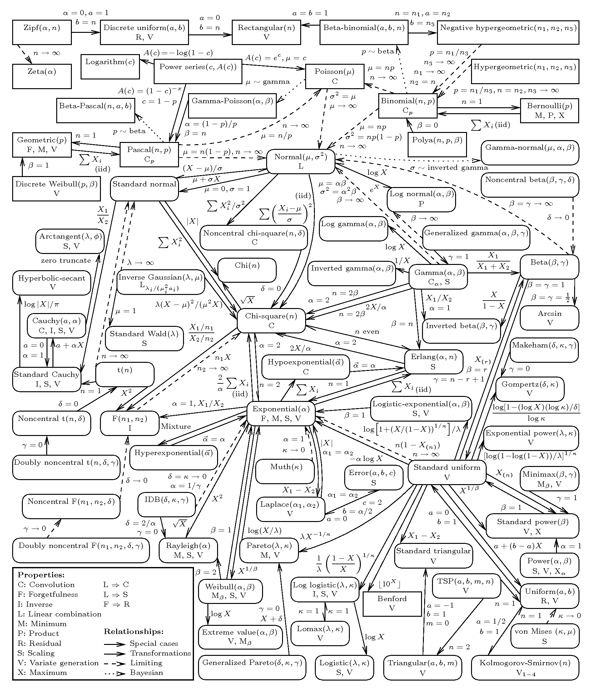
来源：
http://www.math.wm.edu/~leemis/chart/UDR/UDR.html